

Decline:
We have seen that a quantity can increase by a certain percentage over time. In the same way, a quantity can also decrease by a certain percentage.
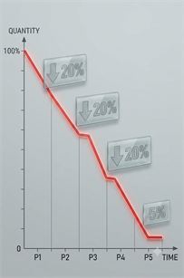
When a quantity decreases repeatedly by a fixed percentage, we call it a decline.
For example,
1. suppose the number of trees in a forest decreases by \(5\%\) every year. The number of trees becomes smaller each year.
A decline of \(\text{r}\%\) means that only \(100 \% − \text{r}\%\) of the previous quantity remains.
Therefore, the remaining percentage is \(100 − \text{r}\) \(\%\).
2. If a quantity decreases by \(8 \%\) , then \(92 \%\) of the previous quantity remains.
\(100 \% − 8 \% = 92 \%\)
Thus, the new value is \(\frac{92}{100}\) \(\times \text{previous value}\).
Decline as a Multiplication:
A percentage decrease can be represented using a multiplicative factor.
If a quantity decreases by \(\text{r} \%\), then \(\text{New Value} = (1− \frac{r}{100}) \times \text{Original Value}\).
Depreciation:
Many objects lose their value as they become older or are used for a longer period. This reduction in value is called depreciation.
For example, a vehicle may lose some of its value because of:
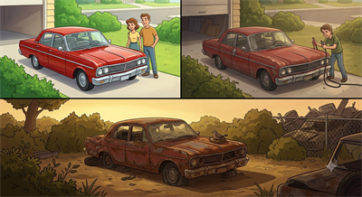
- use over time,
- ageing,
- wear and tear,
- damage, or
- changes in its condition.
Thus, depreciation is the reduction in the value of an item due to use and age.
Repeated Decline:
When a quantity decreases by the same percentage repeatedly, the percentage decrease is calculated on the new value each time, not on the original value.
Formula for Repeated Decline:
Suppose the original value is \(\text{p}\), the rate of decline is \(\text{r} \%\) per period, and the decline continues for \(\text{t}\) periods.
The remaining fraction after each period is \(1-\frac{\text{r}}{100}\).
Therefore, Value after \(\text{t}\) periods \(=\) \(\text{p} (1−100 \text{r})^\text{t}\)
Where,
- \(\text{p}\) \(=\) Principal \ Original value
- \(\text{r}\) \(=\) percentage rate of decline per period
- \(\text{t}\) \(=\) Number of periods
Growth and Decline: A Useful Connection
Growth and decline are opposite processes.
For a growth of \(\text{r} \%\):
For a decline of \(\text{r} \%\):
\(\text{New Value} = \text{Original Value}(1 - \frac{r}{100})\)
Important!
Remember:
1. A decline means a quantity decreases over time.
2. Depreciation is the reduction in the value of an item due to use and age.
3. After a decrease of \(\text{r} \%\), the remaining percentage is \((100 - \text{r}) \%\).
4. A decrease of \(\text{r} \%\) can be represented by multiplying by \(1-\frac{r}{100}\).
5. For repeated decline: \(\text{p} (1 − \frac{r}{100})^\text{t}\)
Tricky Percentages:
Percentages can sometimes look simple but become tricky when a quantity is changed more than once, when we need to find the original value, or when two quantities are compared using different bases.
Successive Percentage Changes:
When a quantity is changed by two or more percentages one after another, the changes are called successive percentage changes.
The important point is that each percentage change is applied to the value obtained after the previous change, not always to the original value.
1. Successive Increase:
Suppose a quantity increases by \(\text{a} \%\) and then by \(\text{b} \%\).
After the first increase, the multiplying factor is \((1 + \frac{\text{a}}{100})\)
After the second increase, the multiplying factor is \((1 + \frac{\text{b}}{100})\)
Therefore, \(\text{Final Value}\) \(=\) \(\text{Original Value} \times (1+100 \, \text{a}) \times (1+100 \, \text{b})\)
2. Successive Decrease:
Suppose a quantity decreases by \(\text{a} \%\) and then by \(\text{b} \%\).
The multiplying factors are \((1 - \frac{\text{a}}{100})\) and \((1 - \frac{\text{b}}{100})\)
Therefore, \(\text{Final Value}\) \(=\) \(\text{Original Value} \times (1-100 \, \text{a}) \times (1-100 \, \text{b})\)
Example:
1. A price increases by \(20 \%\) and then decreases by \(10 \%\).
The second percentage change is calculated on the new value after the first change.
If the original value is \(\text{P}\).
\(=\) \(\text{P} \times 1.20 \times 0.90\)
\(=\) \(1.08\) \(\text{P}\)
Therefore, the final value is \(108 \%\) of the original value.
So, the overall change is an \(8 \%\) \(\text{increase}\).
2. Suppose a quantity increases by \(20 \%\) and then decreases by \(20 \%\).
Starting with \(100\): \(100 \times 1.20 = 120\)
Then, \(120 \times 0.80 = 96\)
The final value is \(96\).
Thus, the overall change is \(100 − 96 = 4\) or a \(4 \%\) \(\text{decrease}\).
The reason is that the \(20 \%\) decrease is calculated on \(120\), not on the original \(100\).
Important!
Successive percentage changes cannot usually be added directly.