

1. Identifying the linear patterns:
Let us consider an example,
A taxi service charges a fixed base fare of \(Rs. 100\) just to start the ride, plus an additional charge of \(Rs. 15\) for every kilometre travelled.
The following steps show how the total fare changes as the distance varies:
For \(0\) \(\text{km}\) (just stepping into the taxi): \(\text{Fare} = 100\)
For \(1\) \(\text{km: Fare} = 100 + 15(1) = 115\)
For \(2\) \(\text{km:}\) \(\text{Fare} = 100 + 15(2) = 130\)
For \(3\) \(\text{km:}\) \(\text{Fare} = 100 + 15(3) = 145\)
Fare calculation breakdown:
| Distance travelled (in km) | \(1\) | \(2\) | \(3\) | ... | \(k\) |
| Total fare paid (Rs.) | \(115\) | \(130\) | \(145\) | ... |
\(100 + 15k\)
|
Mathematical Connection:
If \(k\) is the number of kilometres travelled, the total cost will be \(Rs. 100 + 15k\).
Here \(100 + 15k\) is a linear polynomial in the variable \(k\).
The amount paid increases by the constant value of \(Rs. 15\) for every kilometre travelled.
Such patterns are called linear patterns.
Why is it in a linear pattern?
Every time the distance increases by \(\text{1 km}\), the total fare increases by a constant amount of \(Rs. 15\)
Change in fare \(= 130 - 115 = 145 - 130 = ... = 15\)
Which has a constant difference.
Definition of linear pattern:
A linear pattern is a sequence of numbers where the difference between any two consecutive terms is constant.
In the example above, the relationship between the number of kilometres the taxi travelled and its fare is linear.
2. Constructing Linear Expressions
A linear expression is constructed by the linear pattern formed over the given situation.
Using the example given in the above topic, we get,
The linear pattern as \(100 + 15 k\), where
\(100\) is the fixed charge and \(15\) is the additional charge for each kilometer, k.
Thus, the linear expression can be constructed by,
Linear expression = Fixed Value \(\pm\) (additional value)( chosen variable for the given information)
We use \(+\) sign if there is an increase in the constant value, and we use \(-\) sign if there is a decrease in the constant value.
3. Systematic Representation
A linear relationship represents the relationship between two variables \(x\) and \(y\) can be expressed as,
\(y = ax + b\)
Where \(a\) is the slope(rate of change) and \(b\) is the fixed or initial value (constant).
For the above taxi charge example, we can represent it as,
\(y = 100 + 15 x\)
Where \(y\) is the total charge for the taxi travelled.
and \(x\) is the number of kilometres the taxi travelled.
4. Visualising Linear Relationship using graphs:
Graph of a linear equation in two variables:
The equation of the straight line can be expressed as a line equation in the form of \(y = axe + b\).
To plot a linear equation we need to identify minimum of two points \((x_{1}, y_{1})\) and \((x_{2}, y_{2})\) on the choosen line by taking any two points for \(x\) and calculate the \(y\) values for those points.
We plot those points on the coordinate plane, join them and extend the line in both directions to graph the line.
Example:
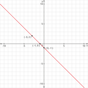
Graph the linear equation \(y = - x- 1\)
Solution:
Given the equation as follows,
\(y = -x - 1\)
Substitute \(x = 0\)
\(y = 0 - 1 = -1\)
Substitute \(x = -1\)
\(y = -(-1) -1 = 1 - 1 = 0\)
Substitute \(x = -3\)
\(y = -(-3) -1 = 3 - 1 = 2\)
Thus, if forms,
| \(x\) | \(-3\) | \(0\) | \(-1\) |
| \(y\) | \(2\) | \(-1\) | \(0\) |
Plotting these points on the graph and connecting them to get a line.
5. Analysing Linear Relationships: Equations & Graphs
Slope and y - intercept:
In the equation \(y = ax + b\),
\(a\) represents the slope (rate of change) of the line, indicating the steepness and direction of the line.
\(b\) represents the y - intercept (starting value) of the given line, indicating where the line crosses the y-axis.
Example:
\(y = 2x + 4\)
Comparing the above equation with \(y=ax+b\) we get,
Slope, \(a = 2\) and
y-intercept, \(b = 4\)
Characteristics of Slope and Y-Intercept:
The Behavior of Slope \(a\)
The slope determines both the direction (growth vs decay) and the steepness of the line.
1. Direction: Positive vs Negative Slope
(i) Linear Growth \((a > 0)\): If the slope is positive, the line goes up from left to right.
Example (Travel Cost):
\(C(x) = 15x + 100\).
Here, the slope is \(15\). For every hour \((x)\) spent traveling, the total cost \((C)\) increases by \(Rs. 15\).
(ii) Linear Decay \((a < 0)\): If the slope is negative, the line goes down from left to right.
Example (Water Tank Leakage):
\(H(t) = -0.25t + 5\).
Here, the slope is \(-0.25\). For every hour \((t)\), the height of the water \((H)\) decreases by \(0.25\text{ meters}\).
2. Steepness: Comparing with the line \(y=x\)
If \(|a| > 1\) (e.g., \(a = 2\) or \(a = -3\)), the line is steeper than the baseline line \(y = x\).
If \(|a| < 1\) (e.g., \(a = 0.5\) or \(a = -0.25\), the line is less steep (flatter) than the line \(y = x\).
(Note: We look at the absolute/numerical value of \(a\), ignoring the negative sign, to determine steepness).
The Behaviour of y - intercept \(b\)
The y-intercept is the point where the line crosses the vertical axis.
Crossing Point: The line always crosses the y-axis at \((0, b)\).
Passing through the Origin: If the y-intercept is exactly \(0\) \((b = 0)\), the equation becomes \(y = ax\). This line passes directly through the origin \((0,0)\), representing a direct proportional relationship.
Visualizing Transformations (Changing \(a\) or \(b\))
Changing \(a\) (Keeping \(b\) fixed): If you alter the slope while keeping the y-intercept the same, the line pivots around its y-intercept. The steepness or direction changes, but it anchors at the same spot on the y-axis.
Changing \(b\) (Keeping \(a\) fixed): If you alter the y-intercept while keeping the slope the same, the line shifts vertically up or down. Because their slopes are perfectly equal, these lines will be parallel to each other and will never intersect.