

Measuring probability objectively
There are two main methods for calculating probability without relying on personal opinion (where someone simply guesses the likelihood based on personal judgment, e.g., "It looks cloudy, so it will probably rain").
(a) Experimental probability
(b) Theoretical probability
(A) Experimental probability
Experimental probability is calculated by actually performing an experiment (or using recorded data) and observing how often an event occurs. In statistics and data analysis, experimental probability is often referred to as relative frequency.
\(\text{Experimental probability} = \frac{\text{Number of times the event occurred}}{\text{Total number of trials}}\)
(B) Theoretical probability
Sometimes we do not need to perform an experiment. If all outcomes are equally likely(a perfectly fair situation), we calculate probability using reasoning. This is called theoretical probability. It is denoted by \(P(\text{Event})\) or \(P(\text{Outcome})\).
\(\text{Theoretical probability}, P(A)\) \(= \frac{\text{Number of favourable outcomes}}{\text{Number of possible outcomes}}\)
Example: A card is chosen randomly from a deck of \(52\) cards. What is the probability of choosing a spade king?
Solution:
Number of favourable outcomes \(= 1\) [There is only \(1\) spade king in the deck of \(52\) cards]
Number of possible outcomes \(= 52\)
\(P(\text{Choosing a spade king}) = \frac{1}{52}\) \(= 0.019\) or \(1.9 \%\)
Analysing statistical data using probability:
In many real-life situations, we cannot predict exactly what will happen, but we can estimate the likelihood of an event by analysing data from observations or surveys. Statistical probability uses information collected from a sample to estimate the likelihood of an event occurring in the whole population.
Example:
A cafeteria owner at a school samples \(50\) students and finds that \(30\) prefer Bhel puri over Pani puri.
Probability that a random student prefers Bhel puri \(= \frac{30}{50} = 0.6\) \((60\%)\)
If the cafeteria has \(300\) regular customers, an estimate of how many prefer Bhel puri \(= 0.6 \times 300 = 180\) students.
This kind of estimation lets businesses plan stock, staffing, or services without surveying every single person.
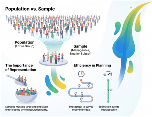
Population: the entire group you are interested in studying (e.g., all \(2000\) students in a school).
Sample: a smaller group taken from the population, used to collect data when studying the whole population is impractical (e.g., asking \(50\) students out of \(2000\) students.)
Sampling: the process of choosing a sample. A good sample should be reasonably large and representative (i.e., it should reflect the whole population fairly, without bias) so that conclusions drawn from it can be reasonably applied to the population.
Statistical probability is essentially experimental probability calculated from sample data, and is often used to make estimates about the larger population.
Difference between experimental and theoretical probability
| Experimental probability | Theoretical probability | |
| Basis | Actual data from performing trials/experiments | Logical reasoning based on a perfectly fair, ideal environment. |
| Formula | \(\frac{\text{No. of time event occured}}{\text{Total observations}}\) | \(\frac{\text{Favourable outcomes}}{\text{All possible outcomes}}\) |
| Can change? | Yes. Different results each time you repeat the experiment, especially with a few trials. | No. Stays the same for a given scenario. |
| Primary use | Real-world applications (e.g., weather forecasting, insurance, quality control). | Games of chance (e.g., dice, cards, coins) where outcomes are symmetrical and fair |
Law of large numbers
Why do experimental and theoretical probabilities often differ? If you toss a coin \(10\) times, you might get \(7\) Heads (an experimental probability of \(70 \%\)), even though the theoretical probability of getting Heads is \(50 \%\).
This is perfectly normal for small sample sizes. As you increase the number of trials (e.g., tossing the coin \(1,000\) or \(10,000\) times), the experimental probability will get closer and closer to the theoretical probability of \(50 \%\). This concept is called the law of large numbers.
Gambler's fallacy
A fallacy is a wrong or mistaken way of thinking. Gambler's Fallacy is the false belief that if a random event has happened many times in a row, the opposite outcome is "due" to happen next.
In reality, each random event is independent, meaning that previous outcomes do not affect future outcomes.
Example: Suppose a fair coin is tossed six times, and the results are \(H, H, H, H, H, H\).

Many people think: "Since heads have appeared six times in a row, tails are more likely to come next."
This is Gambler's Fallacy.
The coin does not remember its previous results.
The probability of getting tails on the next toss is:
\(P(\text{Tail}) = \frac{1}{2} = 0.5\) or \(50 \%\)
The chance remains exactly the same as it was on the first toss.
Fair and unbiased:
A coin, die, or spinner is called fair (unbiased) if every possible outcome has an equal chance of occurring — no outcome is favoured due to physical asymmetry or manipulation.
Random toss:
A random toss/roll means the object is allowed to land naturally without any interference.