

Measures of Central Tendency:
The measures of central tendency are the value that tends to cluster around the middle value of the given set of data.
The following are the three measures of central tendency:
Mean
Mean is defined as the sum of all the observations divided by the total number of observations. It is usually denoted by (x bar).
Therefore, mean \(\frac{\text{Sum of all the observations}}{\text{Total number of observations}}\)
If the number of observations is very long, it is a bit difficult to write them. Hence, we use the Sigma notation \(\sum\) for summation.
That is, , where \(n\) is the total number of observations.
Also, in the case of ungrouped frequency distribution, the formula to find the mean is given by:
Median
Median is defined as the middle value which exactly divides the given set of observations into two equal parts.
- If the number of observations (\(n\)) in the data set is odd, then the median can be determined using the formula, \((\frac{n+1}{2})^{th}\) observation.
- If the number of observations (\(n\)) in the data set is even, then the median is the mean of the values \((\frac{n}{2})^{th}\) and \((\frac{n}{2}+1)^{th}\) observations.
Mode
Mode is defined as the number which most frequently occurs in the given set of data. That is, the observation having the maximum number of frequency is called as mode.
Range
The difference between the highest value and the smallest value in a set of data is the range.
Example:
Consider the following set of data \(2, 7, 8, 6, 10, 5, 6, 8, 2\)
The frequency distribution table will look like the following:
|
Number
|
Frequency
|
|
\(2\)
|
\(2\)
|
|
\(5\)
|
\(1\)
|
|
\(6\)
|
\(2\)
|
|
\(7\)
|
\(1\)
|
|
\(8\)
|
\(2\)
|
|
\(10\)
|
\(1\)
|
From the column 'Number', we know that the highest value is \(10\), and the smallest value is \(2\).
Range \(=\) Highest value \(−\) Smallest value
\(=10−2\)
\(=8\)
Therefore, the range of the given set of data is \(8\).
Construction of frequency distribution table using grouped data:
Class interval and Class size:
Class interval or classes is the difference between the upper limit and the lower limit. The upper limit is the class's highest value, and the lower limit is the class's lowest value.
The difference between the successive upper limits or the successive lower limits is called as the class size or the class width.
Example:
Let us construct a frequency distribution table for the following \(26\) data using tally marks.
\(31, 32, 52, 60, 37, 49, 42, 56, 43, 55, 72, 84, 67, 75, 44, 41, 59, 57, 91, 98, 78, 66, 81, 88, 86, 58\)
Sol:
We can see that the data is very large, and the reader find it difficult to understand it. Hence, let us group the given data.
The minimum value is \(31\), and the maximum value is \(91\). We shall group the data as \(30−39, 40−49, ..., 90−99\), which are called as class intervals.
Consider the classes \(30−39\) and \(40−49\) to find the class size.
Consider the successive upper limits, then the class size \(=40−30 = 10\)
Now, we shall tabulate the data.
| Class interval | Tally marks | Frequency |
| \(30−39\) | 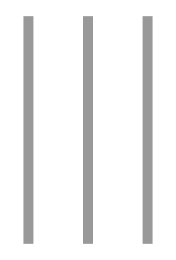 |
\(3\) |
| \(40−49\) | 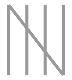 |
\(5\) |
| \(50−59\) | 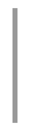 |
\(6\) |
| \(60−69\) | |
\(3\) |
| \(70−79\) | |
\(3\) |
| \(80−89\) | 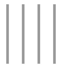 |
\(4\) |
| \(90−99\) | 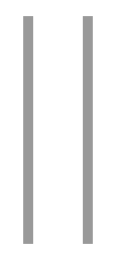 |
\(2\) |
This table is called a frequency distribution table using grouped data.