In an indirect variation, the value of one quantity increases(\(\uparrow\))/decreases(\(\downarrow\)), and then the other quantity decreases(\(\downarrow\))/increases(\(\uparrow\)).
Example:
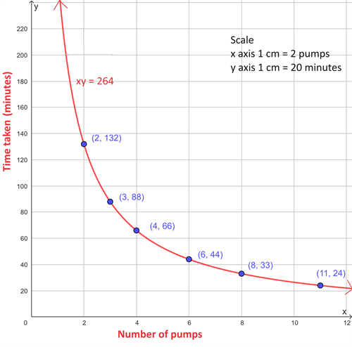
\(2\) pumps working together empty a tank in \(132\) minutes. To fasten the work, more number of pumps have been opened as shown below.
| Number of pumps (x) | \(2\) | \(3\) | \(4\) | \(6\) | \(8\) | \(11\) |
| Time taken (y) | \(132\) | \(88\) | \(66\) | \(44\) | \(33\) | \(24\) |
From the given table, as \(x\) increases, the value of \(y\) decreases. This kind of proportionality is called indirect variation.
Here, \(2 \times 132 = 264\)
\(3 \times 88 = 264\)
\(4 \times 66 = 264\)
\(6 \times 44 = 264\)
\(8 \times 33 = 264\)
\(11 \times 24 = 264\)
Thus, \(xy = 264\). That is, \(264\) is the constant of variation.
Now, let us draw the graph using the given data.
Visualizing Indirect variation:
- We can identify the given data is a indirect variation, if the obtained equation is of the form \(xy = k\), where \(k\) is the constant of proportionality.
- In a graph plotting the obtained equation, we get a curve called rectangular hyperbola.